Smart Energy Management Using Deep Reinforcement Learning

Introduction/Problem

The main motivation for this project stems from my passion for climate tech and my belief that it is a way to ensure a more sustainable future. The paper “Deep Reinforcement Learning for Energy Management in a Microgrid with Flexible Demand” by Nakabi and Toivanen ¹ is relevant to this as it applies reinforcement learning to optimize energy management and resource allocation within buildings connected to an electrical grid. With the introduction and integration of Distributed Energy Resources (DERs) such as wind, solar PV, and natural gas, there is now a need to help manage the loads of the grids by effectively using energy storage systems (ESS) such as batteries ¹. This creates a demand response challenge, where the objective is to utilize the battery-PV system to manage peak loads and decrease reliance on the main grid during high-demand periods. This approach can enhance energy optimization and potentially reduce costs for consumers.

Approach

Nakabi and Toivanen tested seven control algorithms on their environment: DQN, Double-DQN, SARSA, REINFORCE, Actor-Critic, A3C, and PPO. They found that the results of all the reinforcement learning algorithms differed widely in their ability to converge to an optimal policy, with A3C being the best overall when they added an experience replay and a semi-deterministic training phase ¹. Their environment consisted of three control points: a TCL on/off control, ESS charge/discharge control, and an energy grid buy/sell control. They had a multi-agent system, and one of the agents was an ESS agent that had discharge and charge control over the batteries. This was a very complicated setup, and I wanted to see how control algorithms performed in a similar setup. For my project, I focused on a single control point, the ESS agent.

I used the CityLearn environment created by researchers at UT Austin and UC Boulder to create a level of standardization for research in demand response ². The environment I worked with bears similarities to that used by Nakabi and Toivanen in their research, but there are key differences. While Nakabi and Toivanen’s grid utilized wind turbine-based DER, CityLearn’s setup employs building-level solar-PV-based DER. Additionally, the action space in Nakabi and Toivanen’s study was discrete, limited to charge and discharge actions, whereas CityLearn’s action space is continuous, allowing for control in the range of -0.78125 to 0.78125. This discrepancy constrained my ability to effectively experiment with algorithms like DQN, Double DQN, and SARSA. I attempted to integrate weather data from Nakabi and Toivanen, as recommended in my proposal feedback. However, I encountered challenges that I couldn’t overcome, so I opted to use the CityLearn data instead. Although the data itself might be slightly different, my primary objective is to evaluate the effectiveness of different control algorithms in electricity management and demand response scenarios, similar to Nakabi and Toivanen.

The data used in this project is from the 2022 CityLearn Challenge ³, which consists of one year of operational electricity demand and PV generation for single-family houses in Fontana, California from August 2016 to July 2017. I ran a simulation of 7 days with a grid of 2 buildings in my project. I tested the centralized approach, where there is one agent that controls and tries to optimize the storage across all the buildings. CityLearn also allows for a decentralized approach. With the introduction of the environment, the authors of CityLearn also included an example of a multi-agent RL controller using SAC (soft-actor critic) ⁴. To get a sense of the overall performance of the algorithms, I decided to compare it to the performance of SAC. The algorithms I focused on in my project are Advantage Actor-Critic (A2C) and Proximal Policy Optimization (PPO), since these were the best-performing algorithms in Nakabi and Toivanen’s experiments. The observations I used were hour, month, day type, outdoor dry bulb temperature, outdoor relative humidity, diffuse solar irradiance, and direct solar irradiance. I also attempted to implement SARSA and DQN, though I was unsuccessful with DQN. The CityLearn environment offers a discretization wrapper for the action and observation spaces, allowing me to explore their potential for viable results. To proceed, I limited the observation space to the hours of the day, as this approach made the most sense for discretization. The second part of the project was to get a sense of implementing the different control algorithms.

Algorithms Used in the Project

SAC: Soft Actor-Critic

Soft Actor-Critic is an off-policy, model-free algorithm introduced in 2018 by researchers at UC Berkeley ⁵. SAC learns three functions: the policy (actor), soft Q-function (critic), and the value function. The off-policy updates mean that SAC can reuse data, making it more sample-efficient ⁴. SAC also tries to maximize the entropy of the policy along with the rewards. Maximizing entropy allows for more exploration in the policy network ⁶.

A2C: Advantage Actor-Critic

A2C, also known as the Advantage Actor-Critic method, is an on-policy algorithm and a synchronous version of the A3C algorithm. It consists of two networks: the actor and the critic, where the actor learns the policy, and the critic estimates the state value function. The advantage function, which is the difference between the state-action value and state value, is used to update the actor network. The main difference between these algorithms is how they update and process the training data. Since I approached this problem with a centralized agent, I chose A2C over A3C ⁷.

PPO: Proximal Policy Optimization

PPO is an on-policy, model-free algorithm where the main idea is to make sure that during updates to the policy network, the new policy is not too far from the old one. PPO uses clipping to ensure there is not too large of an update ⁸.

SARSA/DQN

Since SARSA and DQN are designed for discrete action spaces, using them with a continuous action space like the one in the CityLearn environment can pose challenges. The CityLearn package provides a discretization wrapper for the action space, which I utilized to test whether DQN and SARSA could produce viable results. Both SARSA and DQN take the state as input and output the Q-values associated with each possible action. SARSA updates its Q-values based on the current action and the action that follows, while DQN uses a target network to stabilize learning and focuses on maximizing future rewards.

Execution

To learn the agent policy for SAC, PPO, and A2C, I used the StableBaseline3 Python library. The CityLearn library also had a normalization wrapper, so I first used this to apply sine and cosine transformations for the time observations and min-max normalize the others. I ran all the algorithms for 20,000 timesteps—each timestep in this environment is an hour, resulting in a total of about 120 episodes. I used a simple MlpPolicy for each of the algorithms with a gamma of 0.99 and default learning rates (0.0007 for A2C, 0.0003 for PPO and SAC). PPO also had clip=0.2. Then, to evaluate the different agents, I ran an episode of deterministic actions to see how well they did compared to each other. I compared their performance by looking at the different KPIs CityLearn tracks, as well as their episode rewards.

For SARSA and DQN, I tried implementing the algorithms using neural networks to approximate the Q-function. The neural network had two hidden layers, and the agent selected actions using an epsilon-greedy approach. (I had issues implementing DQN, so the rest of the discussion focuses on SARSA.) I then ran it for 120 episodes, which was about 20,000 timesteps. To reiterate, I discretized the state and action space and only used hours as observations, so this part of the project was more about understanding the implementation of these algorithms. I then compared SARSA with similar discretized environments of A2C and PPO just to see how well it performed.

Evaluation

Along with the total episodic returns, the agent’s performance is evaluated using six KPIs tracked in CityLearn ⁹. Three of them apply to both building and district (all buildings) levels, and three just to the district level. These are:

• Electricity consumption: the sum of imported electricity into the building, which we want to minimize.
• Cost: the total building-level imported electricity cost.
• Carbon Emissions: building-level carbon emissions.
• Average daily peak: mean of the daily net electricity consumption of all the buildings (district).
• Ramping: the difference between the sum of imported electricity for each timestep (district).
• 1 - Load Factor: efficiency of electricity consumption; we want to maximize this (district).

All these values are normalized with respect to no control outcomes, so any value above 1 means that it does not perform better than a system with no control.

Results

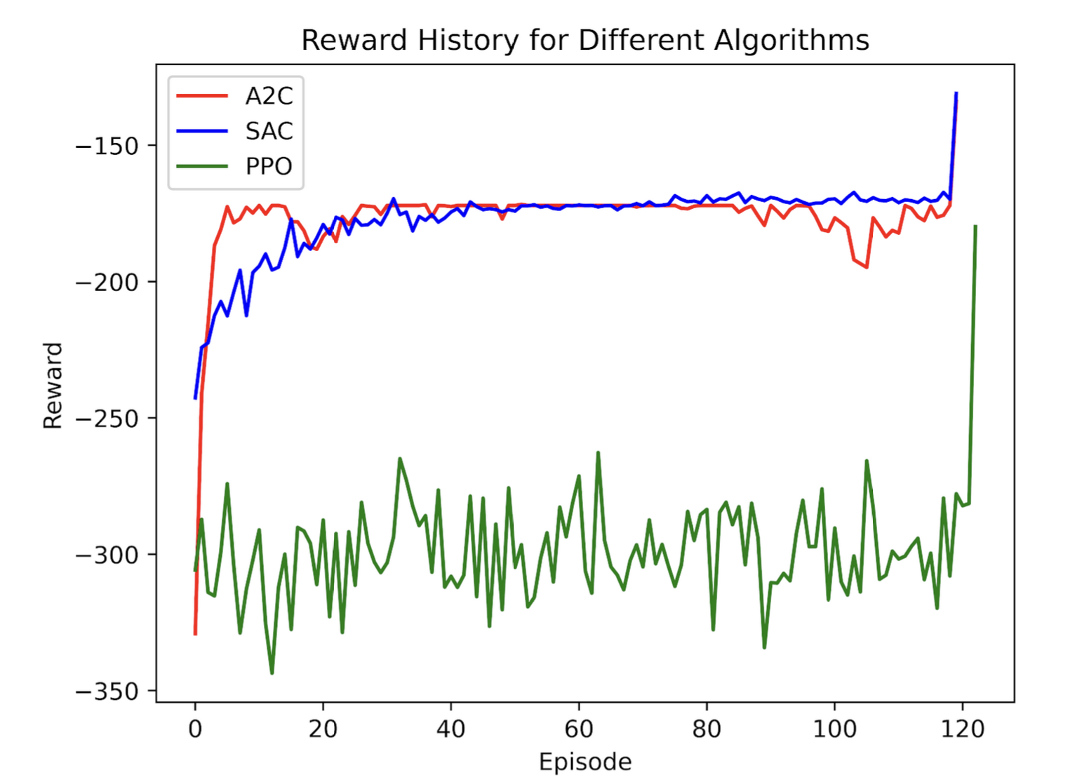
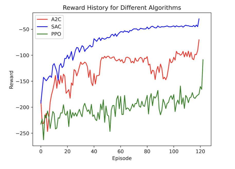
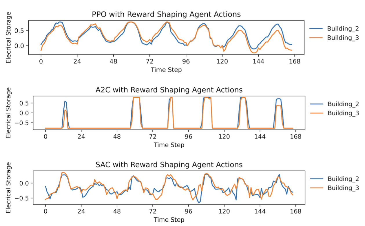
In the initial run of all the algorithms, the reward history showed that SAC and A2C converged, while PPO continued to oscillate. However, an examination of the KPIs revealed that none of the control algorithms performed better than having no control in the environment, as all KPI values were around 1. Notably, Building 2 achieved slightly better building-level KPIs under control. To understand this, I analyzed the agents’ actions: SAC and A2C were discharging the batteries consistently at each timestep for both buildings, while PPO charged and discharged the batteries randomly, leading to less stable results. The SARSA agent, in the discretized environment, also did not perform better than having no control, with KPI values close to 1 as well.

Given these results, it is clear that further tuning and exploration are needed to achieve significant improvements over the baseline. The algorithms may require more sophisticated tuning of hyperparameters, such as learning rates, exploration strategies, and network architectures, to better adapt to the complexity of the environment.

Conclusion

This project provided valuable insights into the challenges of applying reinforcement learning for energy management in microgrids with distributed energy resources. While the initial results showed that the tested algorithms struggled to outperform a no-control baseline in the CityLearn environment, the project highlighted the importance of algorithm selection, environment design, and parameter tuning in achieving optimal results.

Future work could focus on several areas:

1. Hyperparameter Tuning: Experimenting with different learning rates, exploration strategies, and network architectures to improve performance.
2. Algorithm Exploration: Exploring other reinforcement learning algorithms, such as DDPG (Deep Deterministic Policy Gradient) or TD3 (Twin Delayed Deep Deterministic Policy Gradient), which might perform better in continuous action spaces.
3. Environment Enhancements: Integrating additional data sources, such as weather forecasts, and testing the algorithms in more complex, multi-agent setups.
4. Real-World Testing: Applying the trained models to real-world scenarios to evaluate their practical utility in energy management systems.

In conclusion, while this project demonstrated some of the difficulties in applying deep reinforcement learning to energy management, it also laid the groundwork for further research and experimentation that could ultimately lead to more efficient and sustainable energy systems.

References

Nakabi, F., & Toivanen, P. (2020). Deep Reinforcement Learning for Energy Management in a Microgrid with Flexible Demand. Energy and AI. https://doi.org/10.1016/j.egyai.2020.100051 ↩ ↩2 ↩3
Tan, Y., Guan, X., Wu, L., & Li, D. (2022). A Comparative Study on Reinforcement Learning Algorithms for Building-Level Demand Response. Energy and Buildings. https://doi.org/10.1016/j.enbuild.2022.111876 ↩
Vázquez-Canteli, J. R., & Nagy, Z. (2019). CityLearn: Standardizing Research in Multi-Agent Reinforcement Learning for Demand Response and Urban Energy Management. Proceedings of the 2020 International Conference on Autonomous Agents and Multiagent Systems. https://doi.org/10.5555/3398761.3398863 ↩
Raffin, A., Hill, A., Gleave, A., Kanervisto, A., Ernestus, M., & Dormann, N. (2021). Stable-Baselines3: Reliable Reinforcement Learning Implementations. Journal of Machine Learning Research, 22(2021), 1-8. https://doi.org/10.5555/3454287.3454797 ↩ ↩2
Haarnoja, T., Zhou, A., Abbeel, P., & Levine, S. (2018). Soft Actor-Critic: Off-Policy Maximum Entropy Deep Reinforcement Learning with a Stochastic Actor. Proceedings of the 35th International Conference on Machine Learning (ICML 2018). https://doi.org/10.48550/arXiv.1801.01290 ↩
Schulman, J., Wolski, F., Dhariwal, P., Radford, A., & Klimov, O. (2017). Proximal Policy Optimization Algorithms. Proceedings of the 34th International Conference on Machine Learning (ICML 2017). https://doi.org/10.5555/3305890.3306093 ↩
Mnih, V., Badia, A. P., Mirza, M., Graves, A., Lillicrap, T., Harley, T., … & Kavukcuoglu, K. (2016). Asynchronous Methods for Deep Reinforcement Learning. Proceedings of the 33rd International Conference on Machine Learning (ICML 2016). https://doi.org/10.5555/3045390.3045597 ↩
Schulman, J., Levine, S., Abbeel, P., Jordan, M., & Moritz, P. (2015). Trust Region Policy Optimization. Proceedings of the 32nd International Conference on Machine Learning (ICML 2015). https://doi.org/10.5555/3045118.3045133 ↩
Nagpal, S., Zheng, Y., & Candelieri, A. (2022). CityLearn v1.3.0 Documentation. https://citylearn.readthedocs.io/en/latest/ ↩