
Anomaly Detection in Financial Data with Explainable AI
Introduction
Detecting anomalies in financial data can be a valuable tool for investors, financial institutions, and regulators, as these anomalies can indicate potential risks or opportunities. In this project, I worked to leverage Explainable AI techniques to identify and understand anomalies within the financial markets.
Importance of Anomaly Detection
Anomalies in financial data can signal potential risks or opportunities for market participants, helping them make timely decisions. Investors, financial institutions, and regulators can all benefit from the insights provided by anomaly detection, enabling them to make more informed decisions.
Project Objectives
The primary objectives of this project were:
- Anomaly Detection: Identify anomalies in financial markets using deep learning techniques.
- Attention Mechanism: Understand which parts of the input sequence are most relevant for detecting anomalies by incorporating an attention mechanism.
- Explainability: Assess whether the attention mechanism can serve as an explainability tool, providing insights into the specific segments of the time-series data that are significant in detecting anomalies.
Given that this is an unsupervised learning problem, I trained the model using stock market data and cross-checked the identified anomalies with real-world events.
Methodology
Adapting the Neural Network Architecture
Based on insights from the research on “Unsupervised Anomaly Detection in Time Series Using LSTM-Based Autoencoders” [1], I adapted the methodology as follows:
- Layer and Cell Selection: I empirically chose the number of layers and LSTM cells in the neural network architecture to best fit the characteristics of the time-series data.
- Window Size: The window size for feeding the input sequence into the neural network was selected based on the recommendations from this research.
The researchers concluded that the autoencoder-based approach is a powerful method for anomaly detection in time-series data, which aligned with the motivation for adopting a similar methodology in the project. By carefully adapting the neural network architecture, I aimed to effectively identify anomalies in the financial data.
Subset of Empirically Driven Architecture Selection
Without Attention
| Layers | Sequence Length | MSE |
|---|---|---|
| 4 | 5 | 0.8275809288024902 |
| 10 | 9.563321113586426 | |
| 30 | 57.56193542480469 | |
| 3 | 5 | 0.8505892753601074 |
| 10 | 0.754558801651001 | |
| 30 | 10.7001953125 | |
| 2 | 5 | 0.23865096271038055 |
| 10 | 0.2256737947463989 | |
| 30 | 0.6528282165527344 |
With Attention
I tried to improve the reconstruction even more by adding an attention layer in the decoder.
| Layers | Sequence Length | MSE |
|---|---|---|
| 2 | 5 | 0.855551540851593 |
| 10 | 0.18225570023059845 | |
| 15 | 0.38138288259506226 | |
| 30 | 0.43995824456214905 |
Data Pre-Processing
For model training and testing purposes, I did an 85 - 15 train-test split, resulting in 8,755 and 1,546 data points, respectively. I also set aside 10% of the training data for validation during the training phase.
I experimented with different window sizes as input to the LSTM model, along with overlapping and non-overlapping windows. After testing, I found that a window size of 10 (essentially 10 days of data) and non-overlapping windows gave us the best results. Overlapping windows tended to cause overfitting, even with a small number of epochs.
For preprocessing, I normalized the close price of the S&P 500 using Min-Max normalization, which helped make the data more consistent and comparable across different time steps. I used MinMaxScaler from Scikit-learn because it scales the data linearly while preserving the effect of outliers.
Model Architecture
The model consists of the following layers:
- Encoder:
- Encoder Layer 1: 128 Units
- Encoder Layer 2: 64 Units
- Latent Vector
- Decoder:
- Decoder Layer 1: 64 Units
- Attention Layer 1: (q: decoder lstm1, v: latent vector)
- Decoder Layer 2: 128 Units
- Attention Layer 2: (q: decoder lstm2, v: encoder lstm1) (For Visualization)
- Output Layer
In the attention layer, q represents the query vector and v represents the value vector.
I trained the model using the processed training data over 10 epochs, with a batch size of 16 samples. The validation split was set to 10%, and the data was not shuffled during training to maintain the temporal order. I then evaluated and predicted using the test data. Finally, I used the attention scores from the second attention layer to visualize the most relevant parts of the input for anomaly detection.
Results
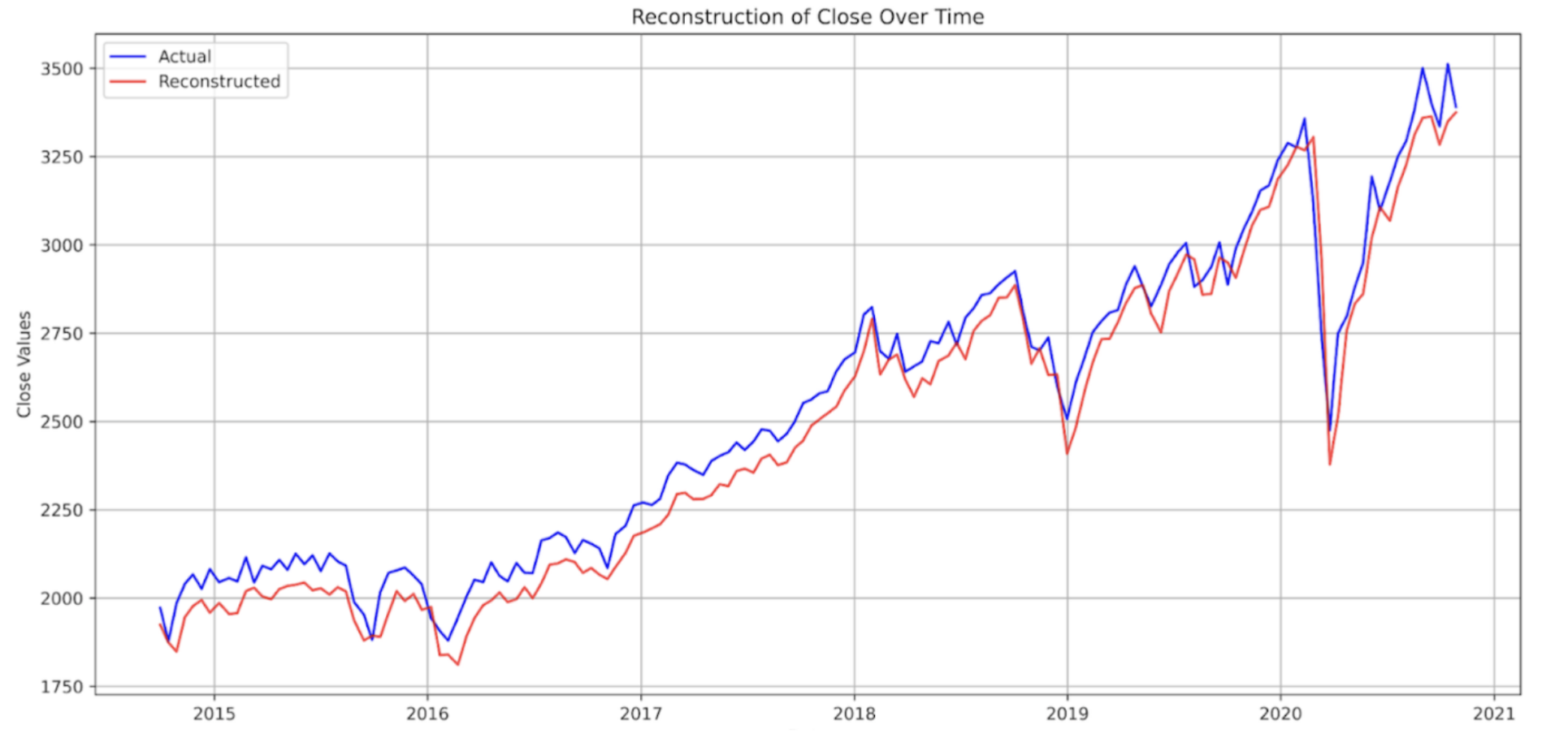
With the described architecture, Iachieved a notably strong reconstruction performance, attaining a Mean Squared Error (MSE) of 0.197367 for the test dataset. Anomalies were detected by evaluating the reconstruction errors against the set thresholds for each time-series window. These anomalies were identified by points surpassing the set threshold.
In the final model iteration, Ifine-tuned the threshold by exploring values spanning the 95th to 99th percentiles of the error distribution. This experimentation led us to select a threshold of 98.5, optimizing the model for anomaly detection accuracy.
When plotting anomalies against the close prices of the stock, Iobserved that anomalous points were detected just before major market fluctuations. For instance, an anomaly was detected at the end of 2018, corresponding to the US-China trade war, which affected the market. Another set of anomalies was detected in late February 2020, just before the market crash due to COVID-19. These findings suggest that the model’s predictions align well with real-life events.
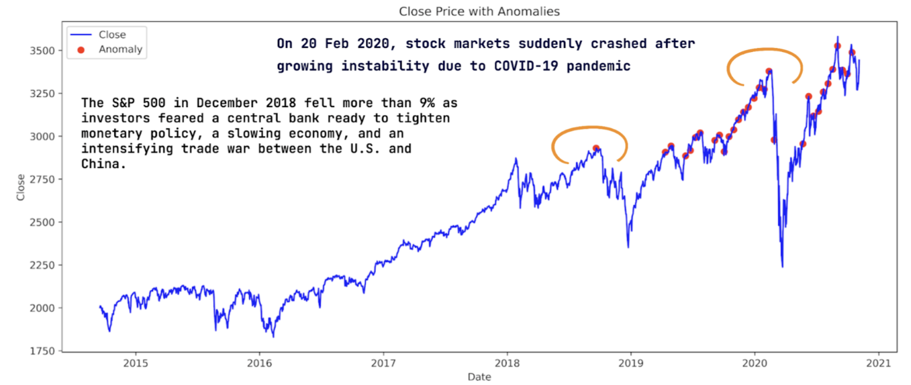
News info source:
Latent Representation
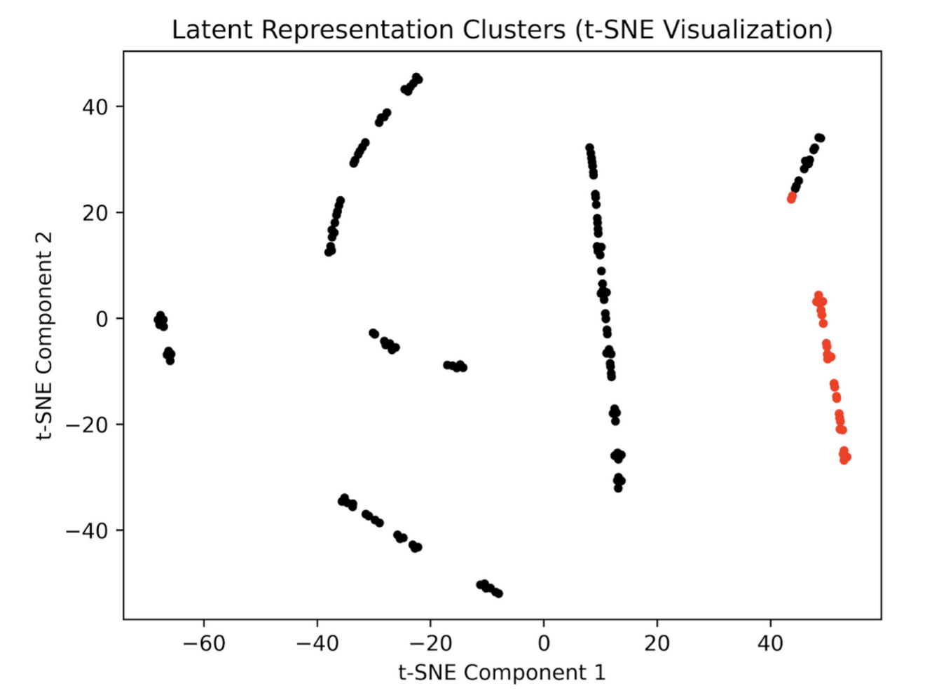
Since this is an unsupervised learning task, I wanted to verify that the detected anomalies were not just random guesses but rather indicative of common underlying patterns in the data. To do this, I plotted the latent representation of the model. In the visualization of the latent space, we can see that the anomalies do in fact cluster together, separate from the main grouping of normal data points. This helps us:
- Confirm the Model’s Effectiveness: The clear separation of anomalies in the latent space suggests the model has effectively learned to isolate anomalous patterns from the normal data.
- Validate Anomaly Significance: The fact that the anomalies form cohesive clusters, rather than being scattered randomly, increases our confidence that they represent meaningful deviations from normal patterns in the data.
Overall, the visualization of the latent space representation provides valuable confirmation that the anomalies detected by the unsupervised model are not arbitrary but rather reflect common underlying patterns that deviate significantly from normal financial market behavior.
Explainability using Attention Mechanism
To assess whether using attention can aid in understanding what parts of the input sequence were relevant for anomaly detection, I plotted heatmaps for the attention scores for each batch. I noticed that the anomalies detected by the model were predicted based on the sequence length rather than identifying specific dates within the window as anomalous.
This hindered the ability to properly interpret the anomaly scores as the anomaly was detected on the first day of the window. I tried reshaping the output from the model and de-batching it before calculating the reconstruction error, but this did not fix the issue. I believe this might be happening because the reconstruction error is higher for the first element in the window, causing the model to struggle to reconstruct the initial input sequence accurately.
Although I was unable to interpret the score due to the anomalies being set to timestep 0, I did notice that the distribution of scores between anomalous and non-anomalous windows varied greatly. Specifically, the scores for the anomalous windows were focused on the last 2 timesteps, whereas the scores for non-anomalous windows were focused on the last 4 timesteps of the input. To check if this difference was significant, I computed the KL divergence of these distributions. I found that the distributions between the two different windows did vary significantly. The difference in the distributions of attention scores between anomalous and non-anomalous windows, as quantified by the KL divergence, suggests that the attention mechanism is capturing some meaningful differences in the input sequences.
KL Divergence Scores:
| Comparison | KL Divergence |
|---|---|
| Anomalous vs Non-Anomalous | 0.06116099 |
| Non-Anomalous vs Non-Anomalous | 0.001801715 |
| Anomalous vs Anomalous | 0.001235715 |
Challenges
One of the first challenges I faced was deciding on the architecture of the neural network. Given the complexity of financial time-series data, selecting the right combination of layers, units, and attention mechanisms required extensive experimentation. I encountered difficulties in balancing the model’s capacity to capture complex patterns without overfitting the data.
Another significant challenge was interpreting the results from the attention mechanism. While attention scores are supposed to help identify which parts of the input sequence are most relevant to the model’s predictions, I found that the scores were heavily skewed toward the beginning of each window. This made it difficult to pinpoint specific days or events that might have contributed to the detection of anomalies. I suspect that this issue may be related to how the model handles the initial timesteps of each input sequence, leading to higher reconstruction errors at the beginning of the window.
I also faced challenges in optimizing the threshold for anomaly detection. Since financial data can be highly volatile, setting a threshold that balances sensitivity and specificity was crucial. I explored various percentiles of the error distribution and found that fine-tuning this threshold was essential for improving the model’s accuracy in detecting meaningful anomalies.
Lastly, validating the detected anomalies against real-world events was both a rewarding and challenging task. While the model successfully identified anomalies that aligned with significant market events, such as the 2018 US-China trade tensions and the 2020 COVID-19 crash, not all detected anomalies corresponded to widely recognized events. This highlighted the importance of contextual knowledge and further investigation when interpreting the results of anomaly detection models.
Conclusion
In this project, I successfully implemented an LSTM-based autoencoder model with an attention mechanism to detect anomalies in financial time-series data. the model demonstrated strong performance in identifying significant market anomalies, and the use of attention scores provided some insights into the underlying patterns in the data. However, the challenges I faced in interpreting these scores and optimizing the model architecture underscored the complexity of applying deep learning techniques to financial data.
Despite these challenges, the project highlighted the potential of using Explainable AI techniques to enhance our understanding of anomaly detection in financial markets. By continuing to refine the approach and address the limitations I encountered, I believe that this methodology can be a valuable tool for investors, financial institutions, and regulators seeking to identify and respond to market anomalies.
References:
Malhotra, P., et al. (2016). Unsupervised Anomaly Detection for Seasonal Data using LSTM Networks. In Proceedings of the 24th ACM SIGKDD International Conference on Knowledge Discovery & Data Mining.